Why Solver Choice Matters in Topology Optimization
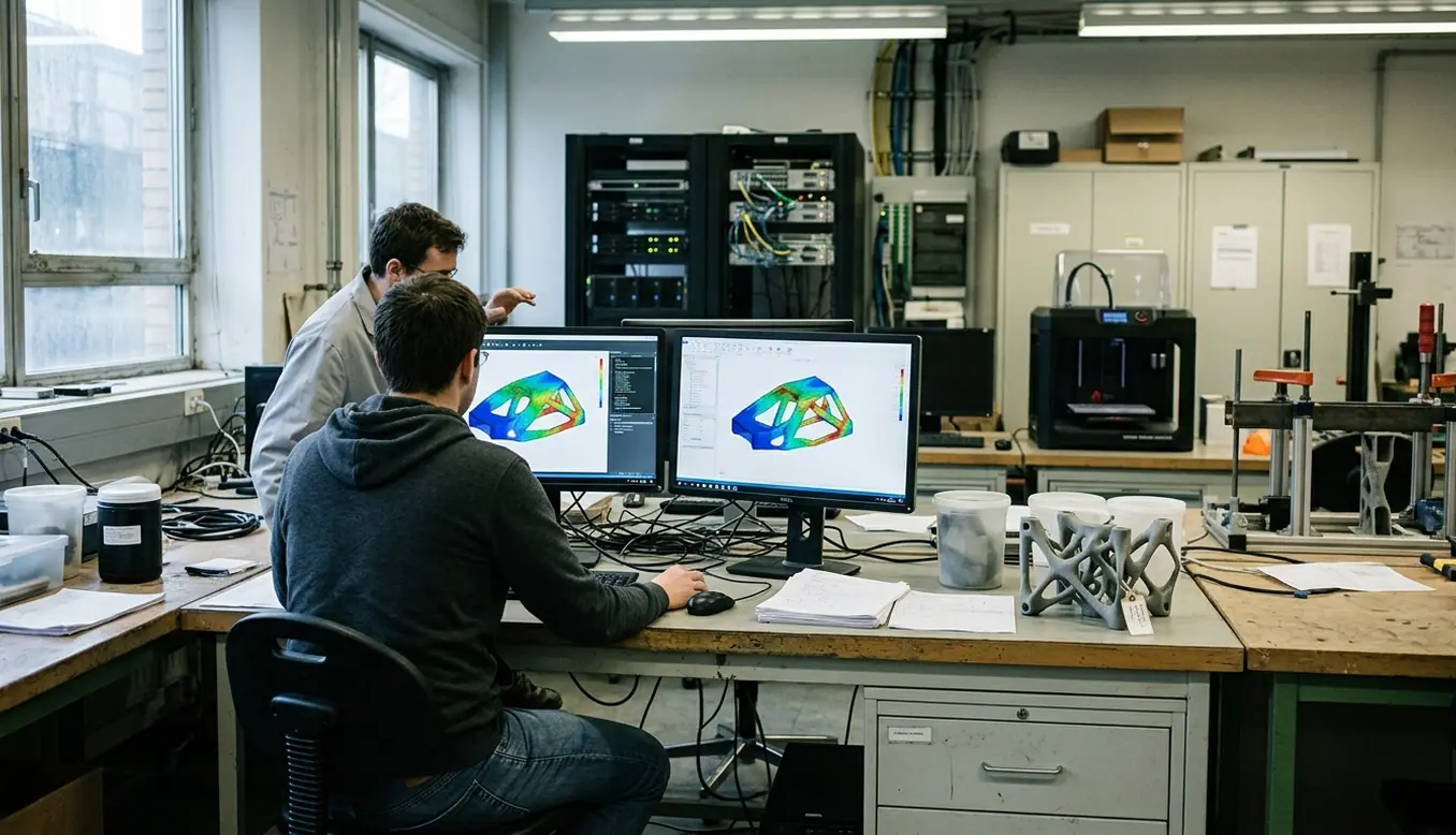
Run the same generative design script on two workstations and you might expect identical output. The benchmark behind this article began when that expectation broke. In late 2022 and the early weeks of 2023, the research team observed persistent discrepancies in compliance minimization results when running identical scripts across different lab machines—same boundary conditions, different final strain energy values.
That is the uncomfortable part. When a solver returns a different structure depending on where it runs, the design itself becomes harder to defend. Engineers treat topology optimization output as an objective answer to a load path problem, yet the answer shifts with the tool.
The need here is straightforward to state and hard to satisfy: reliable design outcomes require knowing how each solver behaves under controlled conditions. A benchmark does not pick a winner. It maps where each method holds up and where it quietly diverges. The remainder of this study documents how that map was built.
Commercial Solvers Selected for Evaluation
The selection committee favored solvers built on established mathematical formulations rather than proprietary heuristics. Two families dominated the shortlist: density-based methods using Solid Isotropic Material with Penalization (SIMP), and boundary-tracking Level Set approaches. Purely heuristic or undocumented optimization engines were excluded, because a benchmark loses meaning when the underlying formulation cannot be inspected.
Procurement and licensing ran through February and into early March 2023.
Application domains differ across these tool families, and that context matters when reading the later results:
- SIMP-based density solvers remain the workhorse for general structural compliance problems, where a continuous density field maps cleanly onto a fixed mesh. They are common in automotive bracket and chassis component work.
- Level Set solvers track explicit boundaries rather than penalizing intermediate densities. Teams reach for them when crisp, manufacturable interfaces matter more than raw iteration speed—aerospace fittings are a frequent use case.
The two families answer the same question with different machinery. That difference becomes visible in the test cases.
Standard Test Cases Employed
To isolate specific stress singularities and load paths, the team selected three classic geometries rather than a sprawling suite. Restraint was deliberate. Three well-understood cases expose more than a dozen poorly characterized ones.
The chosen benchmarks were the Messerschmitt-Bölkow-Blohm (MBB) beam, the L-bracket, and the standard cantilever beam. Geometry standardization ran through most of March 2023. The MBB beam used a 60x20 element base mesh with half-symmetry boundary conditions to reduce computational cost without distorting the load path.
Evaluation criteria centered on two quantities that translate across solvers: compliance, the structural response to load under the optimized layout, and the imposed volume fraction constraint. Compliance minimization under a fixed material budget is the canonical objective, which makes it the natural axis for comparison.
The table below summarizes the geometries and the metric assigned to each.
Standard Benchmark Geometries and Evaluation Criteria| Test Case | Primary Load Path | Key Evaluation Metric | Mesh Resolution (Base) |
|---|---|---|---|
| MBB Beam | Bending under central point load | Compliance minimization | 60x20 elements |
| L-Bracket | Re-entrant corner stress concentration | Compliance under volume constraint | 40x40 elements (minimum) |
| Cantilever Beam | End-loaded bending | Compliance minimization | 60x20 elements |
The L-bracket earns its place specifically because of the re-entrant corner. That geometry produces a stress singularity no solver can ignore, and it sets up an edge case examined later.
Benchmarking Methodology and Controls
A benchmark is only as trustworthy as its control variables. Researchers locked the volume fraction constraint and standardized the penalty factor across every run, so that differences in output traced back to the solver formulation rather than parameter tuning or hardware drift.
Hardware consistency mattered as much as parameter consistency. Every run executed on standardized workstations with dual 16-core processors and 128GB ECC RAM. The computational execution phase spanned roughly April into mid-May 2023. Holding the machine fixed removed the very variable that triggered the original investigation.
Performance was characterized qualitatively rather than through a single composite score. Three dimensions guided the assessment:
- Boundary crispness — whether the final structure resolved into clean solid-void regions or retained ambiguous intermediate material.
- Convergence behavior, how steadily each solver approached a stable layout under fixed parameters.
- Topological stability, whether the resulting structure held its shape when the mesh changed.
Convergence speed itself depends on the optimizer. Solvers using an optimality criteria (OC) method behave differently from those built on the Method of Moving Asymptotes (MMA), and that distinction surfaces clearly once the cases run.
Quick Tip: Before comparing solver outputs, lock your penalty factor and volume fraction first. A mismatch in either parameter will masquerade as a solver difference and waste a full analysis cycle.
Comparative Performance Across Cases
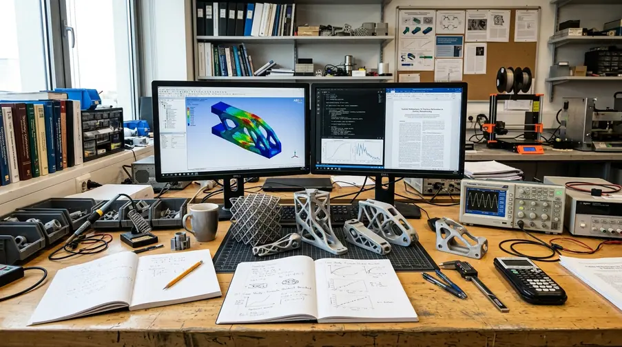
Evaluation involved overlaying the resulting STL files to measure topological deviation between solvers on the same case. The team looked specifically for intermediate density elements—gray regions that signal an incomplete push toward a binary solid-void design. This overlay and analysis phase ran from late May into mid-June 2023.
The clearest split appeared between crisp boundaries and gray transition zones. Level Set outputs produced sharper interfaces by construction, since they track the boundary explicitly. SIMP outputs, depending on penalty handling and convergence, more often retained intermediate densities at structural edges.
The L-bracket exposed a sharper failure mode.
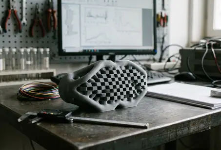
When mesh resolution at the re-entrant corner dropped below 40x40 elements, checkerboarding anomalies emerged—alternating solid and void elements arranged in a pattern that carries no real structural meaning. The corner singularity amplifies this numerical artifact, which is why the L-bracket's minimum mesh threshold was set where it was. Solvers with stronger filtering suppressed the pattern; others reproduced it readily below that resolution.
Convergence speed tracked the optimizer choice rather than the geometry. OC-based runs reached stable layouts on the simpler bending cases with fewer iterations, while MMA-based runs showed steadier behavior on the constrained L-bracket where the design space is more irregular. Neither approach dominated across all three cases—the strength was case-dependent, which is precisely the result a benchmark exists to surface.
For readers extending this work, public topology optimization benchmark studies offer additional reference geometries beyond the three used here.
Scope and Limitations of This Benchmark
This study was deliberately bounded, and the boundaries matter as much as the findings. The scope was restricted to linear elastic materials to avoid the non-linear convergence complexities that would demand an entirely different set of solver parameters. Introducing material non-linearity would not extend this benchmark—it would replace it.
Software versions were locked to their respective early-2023 release builds. The limitation scope was finalized in late June 2023. Solver vendors revise their internal algorithms between releases, so convergence behavior documented here is tied to those specific versions and to the dual 16-core, 128GB hardware configuration described earlier.
Note: The convergence behaviors documented in this benchmark apply strictly to 2D planar stress assumptions. They do not translate directly to 3D multi-load scenarios, where out-of-plane buckling reshapes the design space.
That last caveat is the one most likely to be overlooked. A solver that produces clean, stable 2D layouts may behave differently once buckling enters the picture. Whether the relative rankings observed here survive the move to three dimensions remains an open question—and a fair candidate for the next benchmark.
Summary: Across three standard geometries under controlled hardware and locked parameters, solver outputs diverged most visibly in boundary crispness and in checkerboard sensitivity at coarse L-bracket meshes. Optimizer choice—OC versus MMA, shaped convergence more than geometry did. The findings hold for 2D linear elastic conditions and specific early-2023 builds, not as universal solver rankings.


Comments
Nothing here yet. Add your opinion.
Add Your Thoughts