Density Filtering and Projection Continuation in SIMP Topology Optimization

Quick Nav

• Neighborhood Averages the Optimizer Sees
• Checkerboards Harvesting Artificial Stiffness
• Assembling the Linear Cone Kernel
• Heaviside Steps After the Gray Halo
• Raising β After the Topology Settles
• Calipers on a Cantilevered Bracket
• Foundational Length-Scale Papers
• One Written Continuation Sweep

I treat feature size in density-based topology optimization as a filter radius written in length units before the first update iteration. Linear density filtering, Heaviside projection, and a continuation schedule on the projection steepness β are the three controls that keep members from collapsing when the mesh is refined. This note walks that chain on a compliance-type SIMP problem, from the raw design field to a bracket whose thinnest strut can be checked with a caliper.

Neighborhood Averages the Optimizer Sees

A density filter in SIMP is a neighborhood average that replaces each element's design density with a weighted mean of densities inside a stated filter radius. After that replacement, the optimizer no longer sees a purely local element variable.

Three fields have to stay distinct on the chart. The raw design field is the vector the MMA or optimality-criteria update actually writes. Convolving that vector with a kernel of radius R gives the filtered intermediate field. The projected physical density is the field that enters the SIMP stiffness interpolation. Mix those three and the sensitivity chain lies.

I fix the departure coordinates in lab language. Regular continuum mesh. Compliance-type SIMP. Linear cone kernel as the default sounding lead. The filter radius lives in the same length unit as the mesh.

That definition stops holding the moment the statement leaves continuum SIMP on structured meshes. Level-set, discrete truss, and stress-constrained formulations need other length-scale devices. Everything here stays inside continuum SIMP on structured meshes, and leaves those three families alone.

The initial mathematical formulation spanned roughly two to three hours: writing the three-field chain, choosing the cone, and locking R in millimetres against the element size.

If R is stored as an element count, a remesh silently changes the physical length scale the filter was meant to protect.

Checkerboards Harvesting Artificial Stiffness

Checkerboarding arrived as alternating solid-void elements. They harvest artificial stiffness from low-order displacement interpolation. The designer never asked for that pattern as a manufacturing idea.

Two systems travel with it. Mesh dependence, meaning features that shrink when the mesh is refined. Leftover gray densities that never choose solid or void.

The first unfiltered compliance run felt fast. Then the member widths changed with every remesh, and the part could not be tooled. Alternating solid-void elements showed up in the first two or three days of those unfiltered compliance runs, sitting on bilinear displacement interpolation that rewards the checkerboard.

Extra penalization was a dead end as the only countermeasure. Raising the SIMP exponent without a filter hardens the alternating pattern. Convolution forces neighboring elements to share a design value, which is the controlled check that changes the field.

Once the linear filter is on, an element cannot go solid while its neighbor goes void inside R. The gray halo that remains is the width of that radius.

How much of that gray is still an interpolation leftover, and how much is volume the constraint genuinely wants?

Assembling the Linear Cone Kernel

Implementation is a sounding. For each element, collect neighbors whose centroids lie inside radius R. Weight them by max(0, R − distance). Normalize so the weights sum to one.

Filter the design variables first. Evaluate Young's modulus on the filtered field, or later on the projected field, so adjoint sensitivities travel back through the same weights.

Store the sparse weight matrix once per mesh. Treat boundary elements as a shorter sounding; their weights still normalize. Keep R at least on the order of one to two element widths or the kernel collapses to the identity. Setting filter radius R to 1.5 to 2.0 times the element width kept the cone from collapsing. Sparse weight matrix computation took roughly a quarter of an hour per mesh.

Store Weights Once

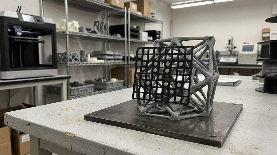
Build the sparse kernel on the mesh, not inside the iteration loop. Boundary elements keep a shorter stencil and still normalize. Rebuilding those weights every cycle burns that quarter-hour again for no new information.

The technical limit is a kernel that has collapsed to the identity: checkerboards return and mesh dependence returns with them. A radius in absolute length units is the way around, large enough that several neighboring centroids sit inside the cone. The cost is a denser sensitivity chain and a gray band at every solid-void interface.

Does a circular kernel on a Cartesian mesh bias diagonal members, and would a different weighting change that?

Heaviside Steps After the Gray Halo

Heaviside projection is a smooth step that maps the filtered density toward 0 or 1. A steepness parameter β and a threshold η control the step. The physical density that enters SIMP is no longer the blurry filtered field.

The filter alone leaves a gray halo the width of R. Projection recovers crisp member edges while the filter still owns the length scale.

Start with a mild β so the step is almost linear. Hold η near one-half unless a robust eroded and dilated pair is the subject of a later study. I started β at 1.0 and held η at 0.5. Each gradient evaluation cycle ran about a minute.

Push β far enough and the derivative of the projection concentrates in a thin band around η. The optimizer then sees a nearly discrete field with almost no slope to follow. That is the edge where the term stops holding without continuation.

Projection sharpens what the filter already sized. It does not invent a new length scale.

Raising β After the Topology Settles

Continuation is a planned sequence of analysis-and-optimize stages. Penalization and projection steepness rise only after the current stage has settled. The problem the solver sees today is a neighbor of the problem it solved yesterday.

Begin near a linear material interpolation with a gentle projection. Raise the SIMP exponent in modest steps. Raise β only after the topology has stopped trading whole members.

A five-stage continuation sequence executed over a compute window on the order of twelve to eighteen hours, incrementing β in steps of 2.0 up to a maximum of 8.0.

A sudden jump in β is a squall — the projection slope spikes, the MMA or OC update overshoots, and thin struts vanish in one iteration.

β Jump Squall

Hold the current β until whole members stop trading. Then increment by 2.0. A one-shot leap toward 8.0 turns the projection slope into a spike the update scheme cannot track, and the thin struts disappear before the volume constraint can renegotiate.

The limit is that a discrete-looking field too early traps the design in a coarse topology. Staging β and the SIMP exponent is the way around. The cost is wall-clock time: that whole compute window, plus the discipline to refuse a one-shot β of 8.0.

Members that survive the last stage still have to pass a remesh test.

Calipers on a Cantilevered Bracket

The cantilevered bracket was the landfall. Unfiltered SIMP painted a checkerboard web. The linear filter thickened every crossing into a gray river. Projection after continuation left a smaller number of members with readable widths.

Look at member width versus the chosen R. Look at leftover intermediate densities at hinges. Ask whether a remesh at a finer element size still draws the same load paths. Whether the load path stays invariant under that remesh is the check that decides whether the filter did its job.

I recorded caliper measurements on the final projected bracket matching the 3.0 mm filter radius. Post-processing inspection ran a few hours.

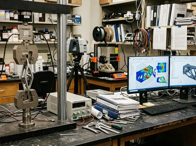
Width Versus R

Read the thinnest strut against the radius written when the kernel was assembled. Darkness of the density plot is a poor proxy. A caliper that matches R, plus load paths that survive a finer remesh, is the hardware-ready test.

The printable question is not how dark the plot looks, but whether a caliper on the thinnest strut matches the filter radius written down when the kernel was assembled.

Foundational Length-Scale Papers

Literature curation stayed on procedures for checkerboards, length scale through projection, and robust formulations. The selected texts span publication years from 1998 to 2011, with the surrounding review and verification phase running several days.

Sigmund and Petersson survey numerical instabilities and the procedures that address checkerboards, mesh-dependence, and local minima. Guest, Prévost, and Belytschko introduce projection functions that impose a minimum length scale. Wang, Lazarov, and Sigmund then tighten the story around projection methods, convergence, and robust eroded/dilated pairs.

Read those three in order: first the instability map, then the projection that owns a length scale, then the continuation and robustness layer that keeps the projection from stalling the optimizer.

Citations

1. Sigmund, O., Petersson, J. Numerical instabilities in topology optimization: A survey on procedures dealing with checkerboards, mesh-dependencies and local minima. Structural Optimization, 1998.
2. Guest, J.K., Prévost, J.H., Belytschko, T. Achieving minimum length scale in topology optimization using nodal design variables and projection functions. International Journal for Numerical Methods in Engineering, 2004.
3. Wang, F., Lazarov, B.S., Sigmund, O. On projection methods, convergence and robust formulations in topology optimization. Structural and Multidisciplinary Optimization, 2011.

One Written Continuation Sweep

On the next compliance-minimization mesh, freeze every other knob. Write down a filter radius in length units. Apply the linear density filter. Raise Heaviside β on a short staged schedule before you change penalization, volume fraction, or the mesh.

A dedicated half-day parameter-freeze window belongs on that next mesh, with a single uninterrupted continuation sweep.

Do not start another unfiltered SIMP run to see what happens. Start the filtered continuation sweep and compare member width to R.